The Minimum Error of Any Classifier: Bayes Error Rate
Bayes error is one of those things that not only sounds good, but is also quite fascinating: it actually defines a theoretical boundary beyond which we cannot go.
And that’s because it confronts us not so much with a technical limitation per se, but with an intrinsic limit of the problem itself, the best that can be achieved given the very nature of the problem from a mathematical and probabilistic standpoint.
An example to better understand
Immaginiamo un problema di classificazione in cui abbiamo:
- X = [x1, ..., xn] n caratteristiche (feature)
- k classi possibili
Let’s imagine a classification problem where we have:
- X = [x1, ..., xn] n features
- k classes possible
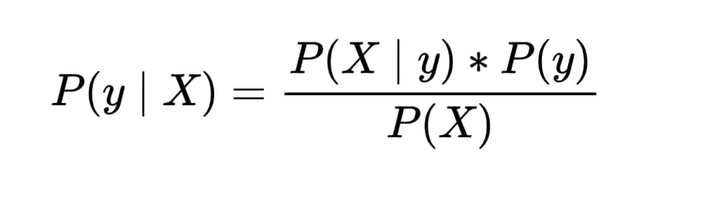
Theoretically, if we knew perfectly how the features X are distributed in relation to the classes y, that is, if we knew P(X | y) — meaning the probability of observing a certain set of features given that it belongs to class y — the prior probabilities P(y) of each class, and the overall probability P(X) of observing those features regardless of the class, then we could use Bayes’ theorem to compute the posterior probability P(y | X):
This would tell us how likely it is that an object belongs to a given class, based on its features X. That would allow us to always classify optimally by choosing the class with the highest posterior probability.
Now, since we’re dealing with probability distributions, choosing the class with the highest probability ensures that we classify correctly most of the time, but it still leaves us with a margin of error.
There’s a detail here that might go unnoticed at first glance but is fundamental: if even knowing the exact probability distribution of a phenomenon I still have a margin of error, it means that this error is unavoidable, dictated by the very structure of the problem.
This minimum theoretical error margin is called the Bayes Error Rate, and it represents the lowest possible error that can be achieved even by a perfect classifier that knows the probabilistic laws governing the phenomenon. And without going into detail, a similar (though not identical) concept exists in regression problems, where it’s called Bayes risk.
In other words, this isn’t an error caused by a bad model or an unsophisticated algorithm: it’s an unavoidable error, caused by the fact that the feature distributions of different classes can overlap.
What does it mean to compute the posterior probability P(y | X)?
Earlier we talked about computing the posterior probability P(y | X). But what does that mean?
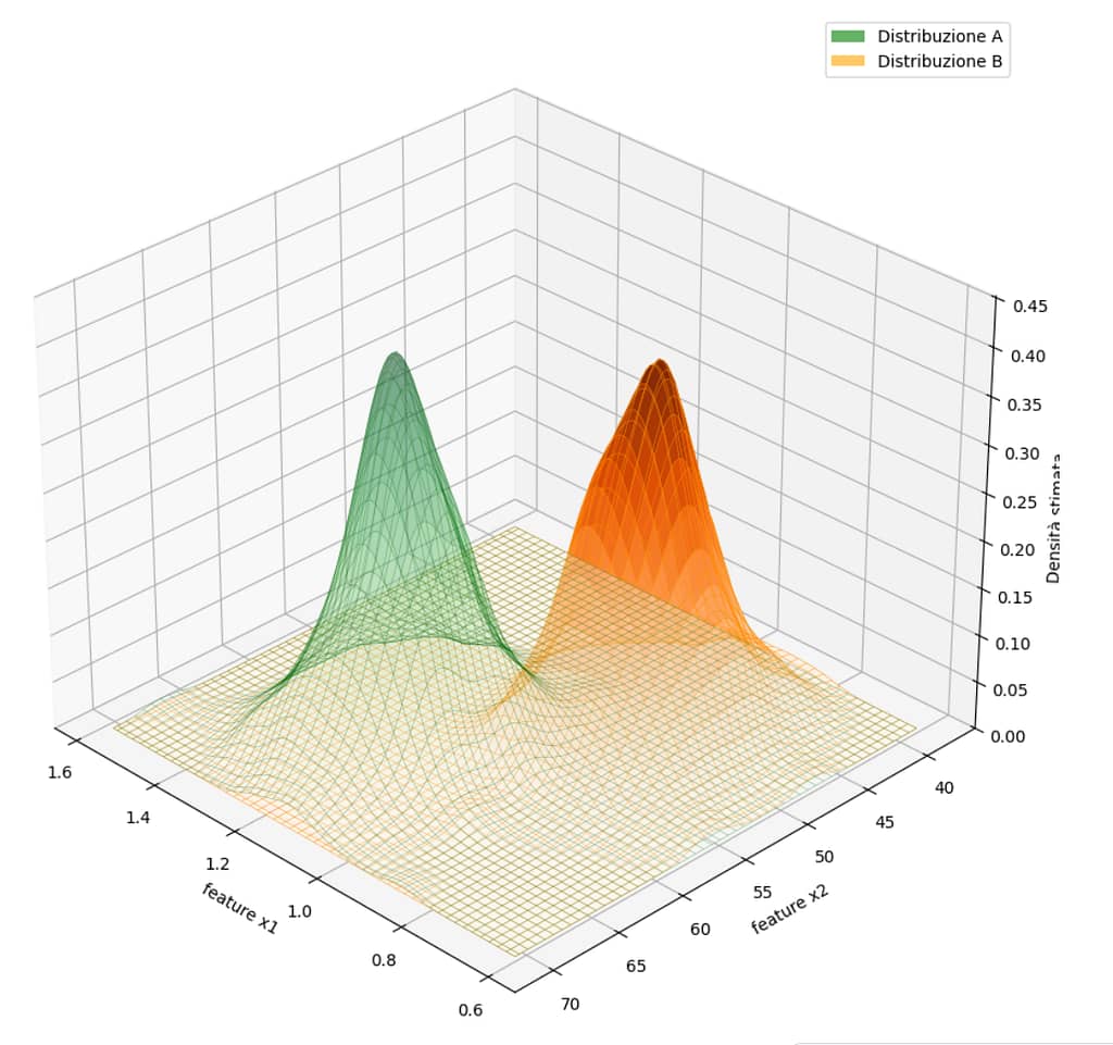
Let’s take a practical example. Imagine we have a classification problem with:
- two arbitrary classes y = [A, B]
- a certain number of features X = [x₁, ..., xₙ]
and we ask ourselves what is the probability that y equals A, knowing that we have "measured" the features X = [x₁, ..., xₙ]
In mathematical terms, we can write P(A | X)
This represents the probability that, given the measurement of the features X, we are looking at an object of class A, and it accounts for the probability of those features occurring when the object is of class A, the prior probability of class A, and the overall probability of measuring X.
But then, if there is a certain probability that we are dealing with an object of class A, it follows that there is also a probability that we are dealing with an object of class B—and clearly this reasoning doesn’t just apply to two classes, but generalizes to multiple classes.
The possibility of error is part of the problem itself
To better understand this concept, let’s forget about A, B, and X and talk about peanuts and pistachios.
Imagine we have a dataset with real measurements of peanuts and pistachios, and suppose for each of them we know the weight (g) and its maximum circumference (mm).
Now let’s suppose we also know exactly how the features [weight, max circumference] are distributed in relation to the classes [pistachio, peanut].
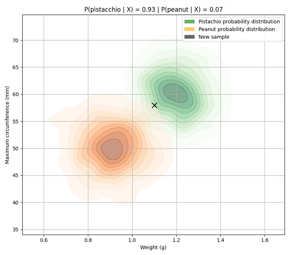
Now a new sample comes in with these measurements:
- weight: 1.1 g
- maximum circumference: 56 mm
👉 The question we ask is: what is the probability that this object is a pistachio, given the features we measured?
Since we’re assuming we know exactly how the features X are distributed in relation to the classes y, to answer this question we just need to calculate the probability that the object is a pistachio given that it has those features, and compare it with the probability that the object is a peanut given those same features.
In practice, we calculate P(pistachio | [1.1, 56]) and P(peanut | [1.1, 56]) and choose the class with the higher probability.
This is called the Bayes classifier (or optimal Bayesian classifier), and it is the classifier with the lowest possible error.
So why do we need Machine Learning then?
So, if using a perfect Bayes classifier would be enough, what do we need Machine Learning for?
Here’s the key point: the Bayes classifier is a purely theoretical concept. It works perfectly only if we already know all the true probability distributions of the problem.
But in practice, in the real world and for real problems, we never have access to these distributions.
They’re hidden in the complexity of reality and the mechanisms that generate our data.
Can’t we estimate them?
In theory, yes. In theory, we could try to estimate these distributions directly by collecting a huge amount of real-world data and empirically observing how features are distributed in relation to the classes, in a purely frequentist way.
However, in practice this approach quickly becomes impractical.
This "frequentist" approach relies on the ability to estimate the underlying probability distributions starting from a subset of the features (the ones we measured).
Now, as long as we’re dealing with one, two, or even three features, a few hundred examples might be enough to get usable estimates. But as the number of features increases, the sample size needed to adequately cover the space of possible configurations grows explosively.
This phenomenon is known as the curse of dimensionality (and it directly affects Machine Learning models as well). It means that in high-dimensional spaces (i.e., with many features), data becomes inevitably sparse, and most of the space remains empty of real observations as the number of dimensions grows.
As a result, as the number of dimensions (features) increases, the space becomes more and more empty, and data increasingly sparse, meaning we need a greater and greater number of features to accurately estimate the distributions needed to directly apply the Bayes classifier—something that, at some point, becomes simply impractical.
But in real-world applications, the number of features can be dozens, hundreds, thousands, or even more. And no, we can’t simply use fewer features, because for real-world phenomena that are extremely non-linear and complex, we need many features to properly map the complexity of the phenomenon.
And this is where Machine Learning really comes into play
In fact, what we do when we train a Machine Learning model is nothing more than trying to approximate these probabilistic relationships — without having to explicitly estimate them in a fully frequentist way.
In other words, we no longer try to directly calculate the full probability distribution of every possible combination of features, because that would require astronomical amounts of data. Instead, we prefer to build a model that, starting from the observed data, learns a compact and generalizable representation of how the features are related to the classes.
This way, we can get close, as much as possible, to the behavior of the Bayes classifier, even without knowing the true underlying distributions.
A Machine Learning model in practice — whether it's a simple linear classifier, a random forest or a neural network — has precisely the task of learning to estimate this distribution, or rather, of getting as close as possible to the real one, hidden in the data.
This means that, ideally, we would like to find those parameters θ such that, given a new element with features X, the estimated probability for the correct class is higher than that for any other class.
Or more formally, if Yi is the correct class, we want that:
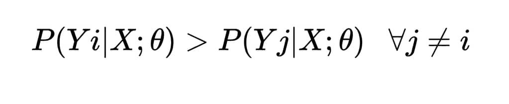
In practice, however, precisely because we never know the true underlying probability distributions, the model does not guarantee this inequality for every single example, but optimizes θ to minimize the overall loss on the dataset, reducing as much as possible the frequency with which this condition is violated. A process that aims to get as close as possible to the theoretical limit established by the Bayes minimum error.
Note that what was just said is not true for all models, but only for the so-called discriminative probabilistic models (such as logistic regression or neural networks with softmax), i.e. those that explicitly estimate the posterior probability P(y | X ; θ). In these cases, the goal of training is precisely to learn a good approximation of these probabilities and then decide based on the highest one.
However, there are also models that do not directly estimate probabilities, such as SVMs, decision trees, or other non-probabilistic discriminative models. These models do not reason in terms of P(y | X), but instead build a decision rule directly — for example, a boundary that separates the classes — by optimizing a different criterion, such as the maximum margin or impurity.
But even if their approach is different, these models still aim to reduce classification error, and therefore — at least in theory — to approach the lower bound set by the Bayes error, which remains valid for any model: precisely because it is a boundary dictated by the nature of the problem, not by the tool used.
Machine Learning was born precisely from the practical need to get close, using the available data and algorithms, to the theoretical limit established by Bayes: that mathematical boundary which represents the best possible outcome given a certain problem.
Training a model means exactly this: finding an efficient way to represent the complex probabilistic relationship between features and target, without having to explicitly observe all possible cases (which would require an unmanageable amount of data).
And it’s beautiful because it reconnects us to the initial concept: even with a perfect model, the minimum error we can ever achieve is set by the intrinsic structure of the problem, by the inevitable overlap of the real distributions.